Chapter 4 Directories and data frames - Week 5 - Workshop 1
This week we don’t have any lectures but we do have an in person workshop. The section to complete this week may be a little more chunky than usual, complete what you can during the workshop and then finish it off in your own time. Do make use of the demonstrators if any of the exercises so far haven’t made sense.
4.1 Data Entry
Let’s have a look at some actual data now, Figure 4.1 shows some lab notes taken during the data collection phase of a small research project to investigate parasite load in 2 small populations of the flour beetle Tribolium castaneum. Each beetle has an ID, a measure of wing casing in mm (which is a good proxy for overall size) and a tally for the number of tapeworm cysticercoids dissected out. In terms of data handling and analysis, we need this data to be stored digitally and we need to have it ordered sensibly in a spreadsheet. We covered what to look for in a tidy, well ordered spreadsheet in our week 3 lecture. Have a go at entering the data from Figure 4.1 into an Excel spreadsheet. When you’re done go to File > Save As…, name your spreadsheet something sensible and make sure you select a sensible place to save it to, where it says File Format: select Comma-separated Values (.csv).
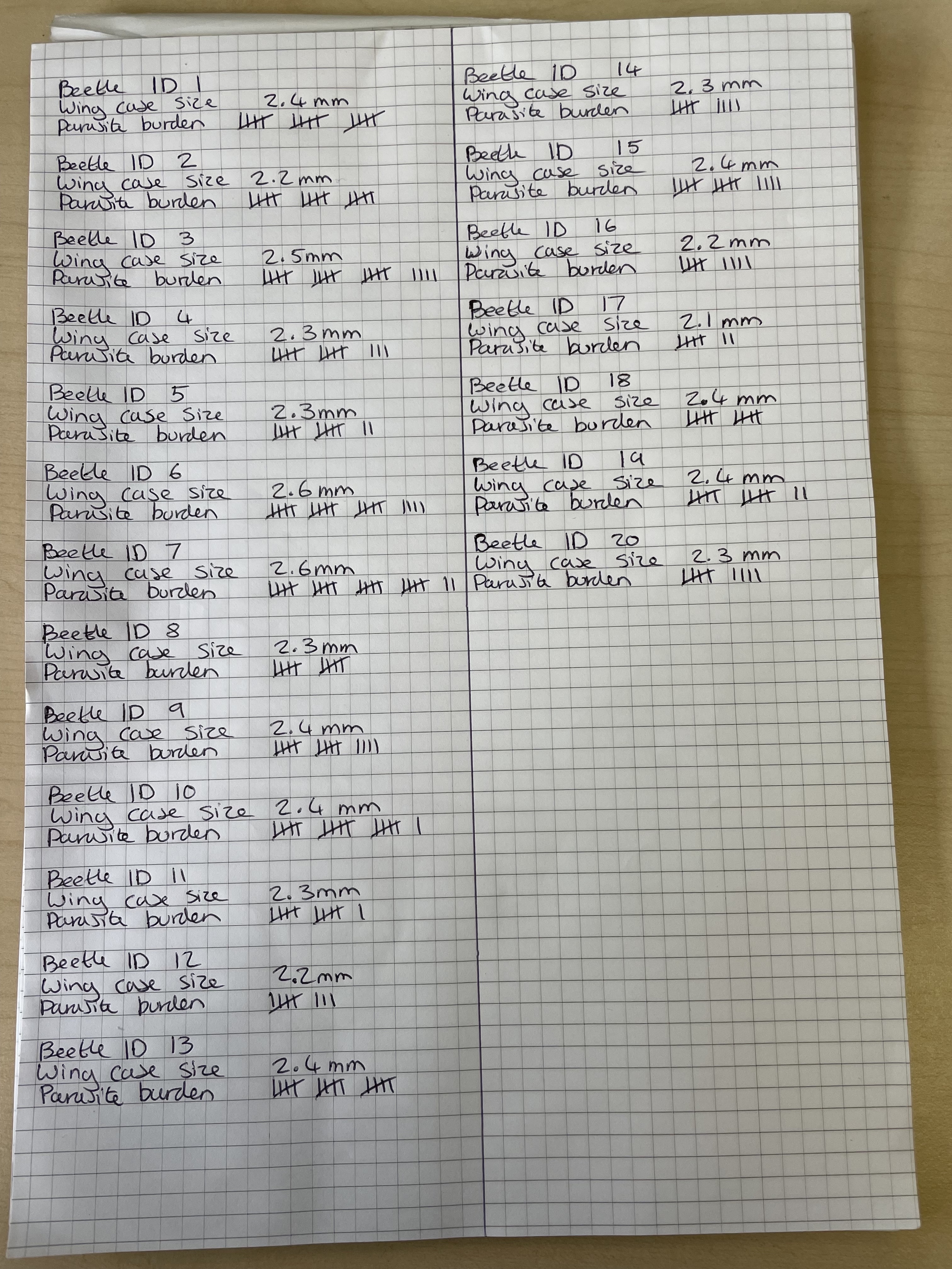
Figure 4.1: Lab notes for wing case size (mm) and parasite burden of 20 Tribolium castanium
4.1.1 A note on naming
While we are on the subject of naming, I am going to take a moment to go over a few good rules to follow. You have just created names for some variables and for a file. You will also frequently have to name folders/directories and objects while working in R, so naming is something that you are repeatedly going to have to do. It therefore makes sense for you to learn how to do it well.
Keep names meaningful - Over the course of your degree you will create a lot of files and folders/directories. You will also frequently be naming data variables and objects. You need to be able to easily recognise what is what so informative names are better then arbitrary names. So
girraffe,elephant,hippoare better names then1,2and3.Make versions obvious - There will be occasions when you want to save new information in a file or object but keep the original untouched. You may be experimenting or you may want the option to revisit to your original work. In these instances it makes sense to save your edits to a new version of the original file or object. If you do this and especially if you are sharing it with others make it clear. I tend to add my initials and a version identifier (e.g. eb_v1, eb_v2) as a suffix to the file name.
Keep names short - Typing takes time, its boring, and the more you type the greater the risk of a typo. So keep names short. So
trunk_lengthis better thanelephant_trunk_length_cm, there is important information in the second name but you can store this as a comment or a note.Avoid spaces - Lots of software packages hate spaces, including R. If you can get out of the habbit of using spaces and instead use
_your future self will thank you.Abide by the rules for R - R does have some rules of its own for naming. Names must not start with a number, but numbers may be used provided the first character is a letter. You can also use
.or_, but avoid spaces at all costs. You may use upper or lower case letters, but remember R is case sensitive so will seeElephantandelephantas different. I try to keep to a lower case and use_instead of spaces, it keeps everything uniform and saves me time (this style is known as snake_case).
Now go back to your spreadsheet, do your variables and file names follow a sensible naming convention?
Make sure you have a demonstrator check your work before moving onto the next step.
4.2 Setting up your R workspace
This is a new piece of analysis, we will be carrying forward principals from the previous chapters but scripts and data will be new. So its a good idea to start with a fresh clean workspace. So lets set up a new project in posit Cloud, follow the steps from Chapter 2 if you cant remember how to do this and name this project tribolium_parasites. Its always good to keep a well organised tidy workspace, generally I will start a new project in posit Cloud if I am working on a new series of questions with a new data set or sets.
For this project you need to make sure two packages are installed. Copy the following directly into your console.
We will be moving towards doing some more comprehensive data handling so setting up your workspace is going to become more and more important. If you can get into the habit of setting up your workspace properly at the start of each project you will thank yourself later. A well developed project will contain several files including;
- Input data
- Scripts
- Outputs
Under Files in the bottom right panel create a New Folder, for each of the following;
- data
- scripts
- figures
Make sure you copy the names over exactly, or some of the commands that we will be using later wont work
A tidy workspace will help you find the things you need when you need them and will reduce the risk of loosing things.
4.2.1 A note on directories and their structure
Working with text based interfaces like R, where you are writing and running commands, means that we need to have some understanding of the underlying computer architecture. You need to have some appreciation for how files are organised within folders/directories and why its important to know which directory you are working from with R.
Under Files in the bottom right panel of your screen you will see a file with the ending .Rproj. This is an R project file which tells R where you are working in the server. It means that R will automatically treat your project location as the working directory. If you wish to access files in any of the folders you have just created you will need to tell R the path that it needs to follow in order to access these files. There are two types of path;
- absolute paths, which refer to the same location in a file system relative to the root directory (don’t worry if that doesn’t make too much sense at this stage). For example, in Figure 4.2, if you wanted to access files in the
/workdirectory but were already in any of the other directories like/dev, an absolute path would work from wherever you were working this would be/home/jono/work. - relative paths, which refer to a location in the file system relative to the directory you are currently working in. For example, in Figure 4.2, if you were working in the
/homedirectory and wanted to access files in/worka relative path would look likejono/work. This is fine from the/homedirectory, but the path would not work if you were working in, for example/lib.
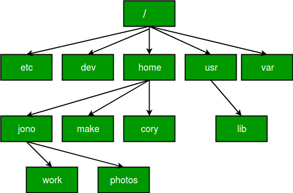
Figure 4.2: Absolute vs Relative Paths
Here we will only be dealing with relative paths because you will always be working from within your R project directory. So for example if you wish to access a file in your data folder in the R project you would need to provide the path ("data/any_sub_folders_you_may_have_made/the_file_you_wish_to_access"). We will do this in the next step so don’t worry if you don’t quite get it yet.
4.3 Setting up your script
Right OK, enough theory, lets start setting up your script. Create a new R script by clicking on the icon with a little green plus, below File in the top left of the posit Cloud window and select R Script. Call your new script tribolium_parasites. Its always good to add a few lines of description at the start of your script, this tells your future self and anyone else what the script is doing. Copy over the following.
# An analysis of parasite abundance between male and female tribolium beetles from two thermal treatments (30 and 35 degrees centigrade)
# Your name
Then we need to load any packages that we might want to use, copy over the following;
4.4 Importing data
Lets import your data set. Go into your data folder within Files, click Upload and select your newly made .csv file. Once its uploaded you should be able to see it under data/ in the bottom right panel.
Now we need to tell R to read your .csv file.
# Read the data from the .csv file in the data folder into my project
tribolium <- read_csv("data/your_file_name.csv")
R should respond with this;
> tribolium <- read_csv("data/tribolium.csv")
Rows: 20 Columns: 3
── Column specification ───────────────────────────────────────────────────────────
Delimiter: ","
dbl (3): beetle_id, wing_case_size, parasite_burden
Here R has told us that there are 20 rows and 3 columns in our data set, it has indicated that it has used comas as a column deliminator and that all the data are dbl (short for double), which means each column contains numbers. You should also be able to see tribolium in your Environment under Data.
If you have errors, make sure your file name and path are input correctly.
Lets have a look at our data to make sure it looks as we expect it to, try this;
We can see for ourselves that R has correctly read our data.
4.5 Creating tibbles
So we have successfully imported data into R from a .csv file and stored it as a data frame which is a type of two dimensional array. Tibbles are a type of data frame as well, these can be useful if you want to type your data straight into R, or if you have more information to add to a pre-existing data frame. For example, we also have some additional data on the sex and treatment conditions of the Tribolium beetles. So lets create a tibble, add the following to your script;
# First of all lets create some variables
beetle_id <- c(1:20) # Notice that this notation will create of a list of numbers 1 to 20
sex <- c("F","F","F","F","F","M","M","M","M","M","F","F","F","F","F","M","M","M","M","M")
treatment <- c(35,35,35,35,35,35,35,35,35,35,30,30,30,30,30,30,30,30,30,30)
Now we neet to turn our new variables into a data frame
Try using head() to check your new tribolium_extras data frame.
4.6 Renaming variables
It may be advantageous to have all the data from both of our data frames together, we can use another function to do this. However first I would like everyone in the class to have the same variable names, this will help us later on but also sometimes its useful to change headings in R. Add the following to your script and run it, make sure you edit it to match your variable names.
# Renaming some variables in your original data set
tribolium <- tribolium %>%
  rename(beetle_id = your_variable_name_here)
# Check how your data frame now looks
head(tribolium)
Side Note you may have noticed the %>% expression, this is known as the forward pipe operator and allows you to chain together commands (rather like the
+we covered in Chapter 2 when usingggplot). This is a very simple use of it but it is piping your data frame forward to the rename function.
Hopefully the column containing your beetle IDs is now labeled beetle_id. Use the same set of commands to rename your variables for beetle wing case size and parasite load. Call the variables wing_case_size and parasite_burden instead.
Now we can merge our two data frames.
# Merge data frames
tribolium_combo <- merge(tribolium, tribolium_extras, by = "beetle_id")
# This merge function combines both of your data frames but matches rows by beetle_id
Take a look at your new data frame now with the head() function, and lets try one more command to do one last check on your data. Try this;
This command will show you something like this;
>glimpse(tribolium_combo)
Rows: 20
Columns: 5
$ beetle_id       <dbl> 1, 2, 3, 4, 5, 6, 7, 8, 9, 10, 11, 12, 13, 14, 15, 16, 17…
$ wing_case_size  <dbl> 2.4, 2.2, 2.5, 2.3, 2.3, 2.6, 2.6, 2.3, 2.4, 2.4, 2.3, 2.…
$ parasite_burden <dbl> 15, 15, 19, 13, 12, 19, 22, 10, 14, 16, 11, 8, 15, 9, 14,…
$ sex             <chr> "F", "F", "F", "F", "F", "M", "M", "M", "M", "M", "F", "F…
$ treatment       <dbl> 35, 35, 35, 35, 35, 35, 35, 35, 35, 35, 30, 30, 30, 30, 3…
Once again we can see that four of our variables have been interpreted by R as being <dbl> vectors, R has identified them as being numeric. One of our variables has been identified as being a <chr> (short for character) vector, so R knows that this variable contains letters or words.
You may now wish to export your new combined data frame as a .csv file. You can do this by running the following command;
# Save your combined data frame as a .csv file (which you could download) to your data folder
write.csv(tribolium_combo,"data/tribolium_combo.csv", row.names = FALSE)
Well done everyone, you have successfully entered your data and uploaded it to posit Cloud as well as making some small adjustments to the data frame and doing a first pass quality check! There are more checks we could have run, and we will revisit this later in the course when we look at some larger data sets. But we will leave this here for now, next week is reading week and the week after we will start looking at checking our data dimensions.
4.8 References
Firke, Sam. 2021. Janitor: Simple Tools for Examining and Cleaning Dirty Data. https://github.com/sfirke/janitor.
Wickham, Hadley, Mara Averick, Jennifer Bryan, Winston Chang, Lucy D’Agostino McGowan, Romain François, Garrett Grolemund, et al. 2019. “Welcome to the tidyverse.” Journal of Open Source Software 4 (43): 1686. https://doi.org/10.21105/joss.01686.
Wickham, Hadley, Romain François, Lionel Henry, and Kirill Müller. 2021. Dplyr: A Grammar of Data Manipulation. https://CRAN.R-project.org/package=dplyr.
Wickham, Hadley, Jim Hester, and Jennifer Bryan. 2021. Readr: Read Rectangular Text Data. https://CRAN.R-project.org/package=readr.