Chapter 2 Introduction to R and posit Cloud - Week 2A

You should aim to complete this chapter in Week 2, Semester 1.

2.1 What is R and posit Cloud?

So hopefully you have read through Chapter 1, where R and the posit Cloud interface were introduced in this module. But what really is R and what is the difference between R and posit Cloud?

Essentially R is a programming language that is commonly used in statistical computing, data handling, data visualisation and data analysis. Posit Cloud is a cloud based interface for a piece of software called RStudio (we wont be using the non cloud based RStudio in this sub-module, so we wont explore this software further here). Posit Cloud uses the R programming language but has a nice user friendly interface and is a great tool for learning how to conduct analysis in R.

We are using the posit cloud rather then RStudio because it means that no one has to worry about installing extra software on their own computers and everyone will be working with the same software versions. You will all need to create your own free accounts on posit Cloud, but first have a look at the short video below introducing you to the interface.

Now that you’ve watched the video, create your own Free posit Cloud account here.

2.2 A warning on managing your work flow

Your free posit Cloud account comes with some restrictions which you should be aware of. These are;

• You may have up to 50 projects in total
• You are limited to 25 project hours per month
• You have up to 1GB of RAM and 1 CPU per project

For the purposes of our work here these restrictions should not be a problem. But I strongly suggest you don’t leave your coursework to the last minute. If you try and pack in a whole semester or years worth or material into a single month, you will exceed those 25 project hours. There are some options of last resort should this happen, you could install RStudio on your desktop for example, or set up an alternative posit cloud account with an alternative email address, but things will get complicated. Lets avoid that where we can! There are some ways you can increase the efficiency of your workspace which are documented below in section 2.4.

2.3 Creating your first posit Cloud Project

Once you have created an posit Cloud account you should be presented with this window

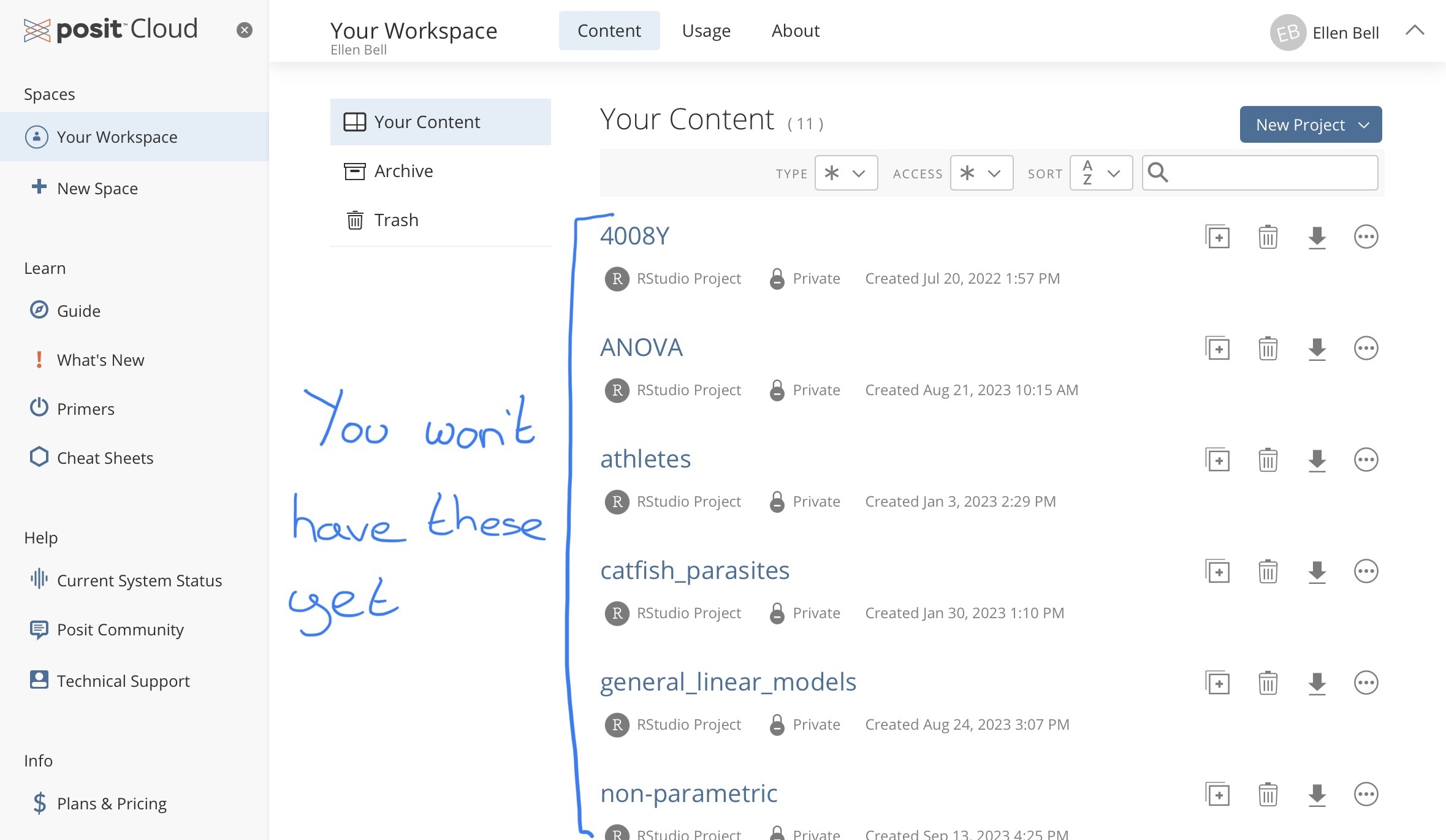
Figure 2.1: Your workspace in posit Cloud

Under Spaces go to Your Workspace and under Projects create a New Project > New R studio Project.

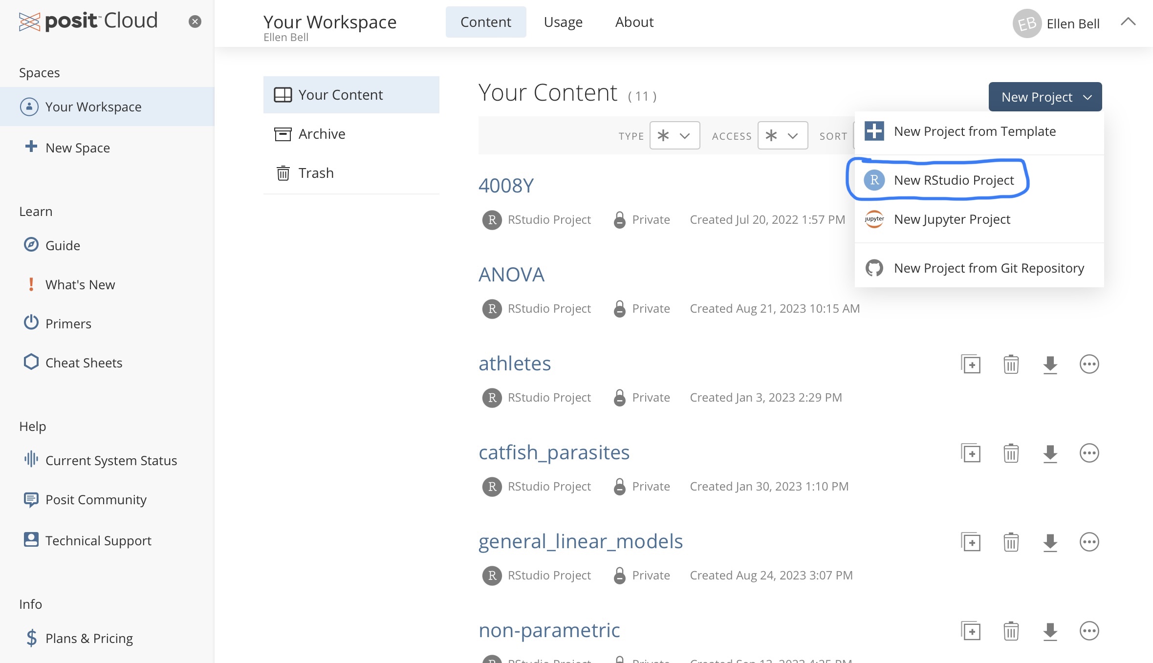
Figure 2.2: Creating a new project in posit Cloud

Lets name this project testing_R, notice that I have no spaces in my project name. Instead of a space I have used an underscore, there are a number of good habits you should try and adopt when project or file naming and not including spaces is one of them, we will go over this in more depth in lectures and later chapters. You can rename your project by clicking on Untitled Project at the top of the window, and typing in your new project name.

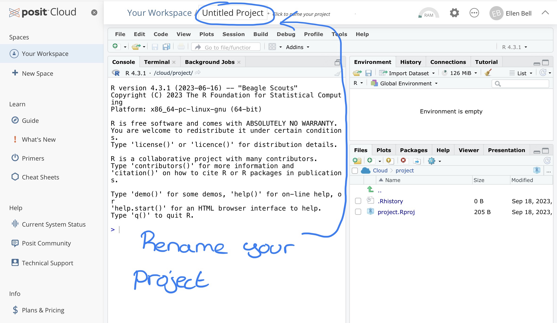
Figure 2.3: Renaming your project

You will see that your new project has three panels with tabs showing the Console, Environment and Files for your project.

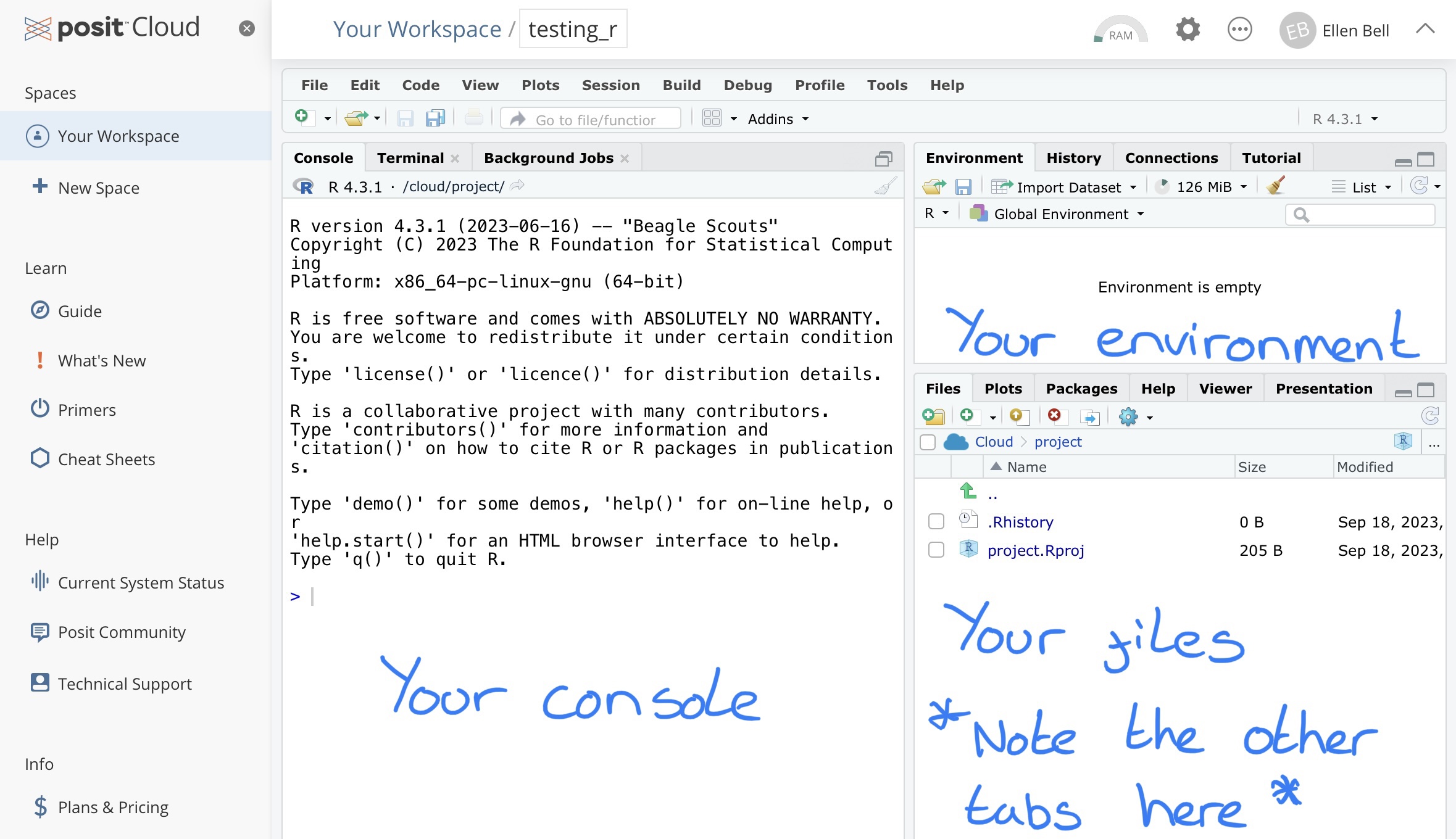
Figure 2.4: The three basic panels of an R Studio workspace

2.4 Maximising the efficiency of your workspace

We know we have limited project hours on our free posit Cloud accounts to reduce your resource usage. In your project, go to settings (the cogwheel sign), Resources, and drag all of the sliders down to the minimum setting, apply the changes, this will mean the project has to restart. This will mean that running the project for 1 hour will consume 0.5 project hours. We wont be doing anything particularly computationally intensive so there is no need for RAM of CPUs to be higher.

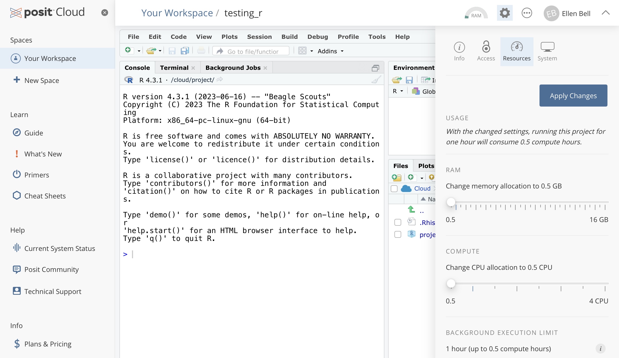
Figure 2.5: How to make your project more efficient

2.5 Entering commands directly into the consol

Lets start by playing with some commands in the console. Type or copy and paste the simple calculation (or command) shown below, into the console. Your text should appear next to the > symbol. Press Enter on your keyboard, this will instruct R to run the command.

5 + 9

The two final lines of your output should look like this:

> 5 + 9
[1] 14

So… your initial command 5 + 9 is shown after the >, symbol and the resulting output from R is shown after [1]. Don’t worry too much about the syntax of > and [1] here. You can think of > as meaning that R is ready to receive a command and [1] as R telling you that the answer to the first part of your question is here (in this case 14).

Try out some other commands… What happens when you input the following?

362 * 12

55 / 5

(40 / 990) * 100

4^2

See if you can work out what 30% of 735 is using the R console

2.6 Sending commands down to the console from an R script

I have already mentioned the reproducibility factor as an advantage of using posit Cloud. This is because you can record and run all of your commands from an R script within posit Cloud. This means that you have a written record of your analysis workflow, what you did to your data at which stage, and you can do all of this without altering the original data files! This is super important because it means that if you revisit your work in a few weeks/months/years you can see exactly what you did AND if someone else needs to rerun any of your analysis or use your workflow on some other data, they can!

So lets go about setting up your new script. You currently have three panels in posit Cloud. If you go to file > New File > R Script a new panel will open.

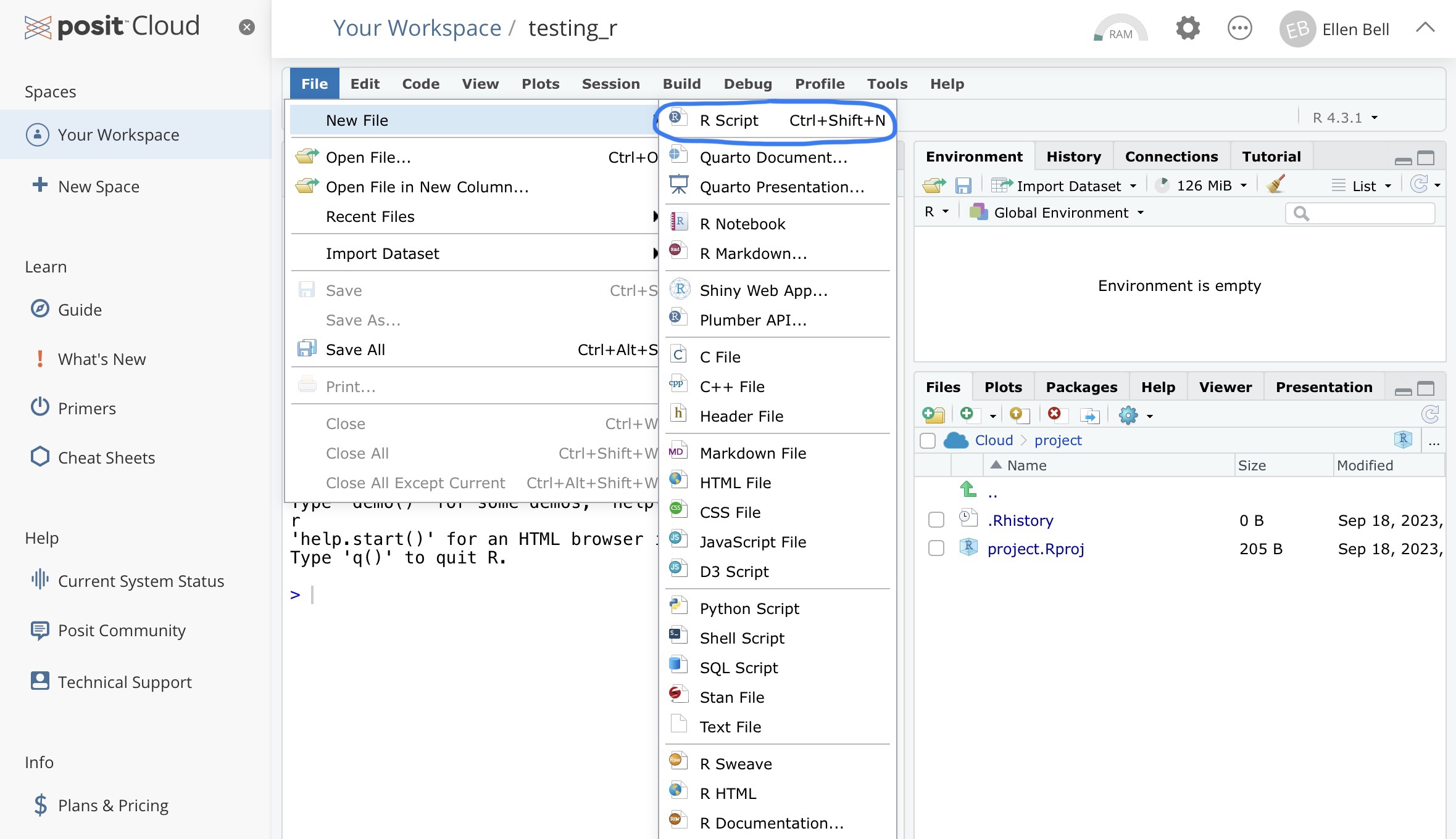
Figure 2.6: How to create a new R script

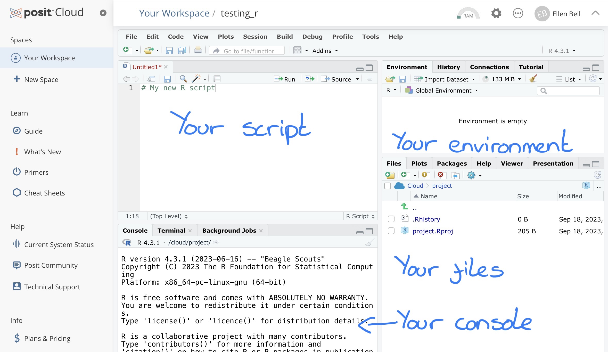
Figure 2.7: The four panels of an R Studio workspace

This new panel is essentially a text file where you can write your commands into a script and then send them down to the console when you want to run them. Lets have a play. Copy the below into your new R script.

362 * 12

55 / 5

(40 / 990) * 100

4^2

These are all commands you have run before but now if you save your script you will have a text based document with your progress saved. It doesn’t make a huge amount of sense to do this now because these are just a un-associated set of calculations and we are just playing with the interface, but you could if you wanted to.

Ok, so now we are ready to execute our commands. You can do this with each calculation individually, line by line, or you can run the whole script.

To run your script line by line, place your cursor on the line you wish to run and you can either;

• Click on the Run button on the top right of the script panel
• Press ctrl + Enter (or Command + Enter on mac)

Or if you wish to run the entire script you can either;

• Manually highlight the script and click the Run button or press ctrl + Enter (or Command + Enter on mac)
• Press ctrl + A (or Command + A on mac) and then click the run button or press ctrl + Enter (or Command + Enter on mac)

2.7 A note on comments

When you are writing a script you can leave notes for yourself. This can be extremely useful if you need reminding on what a particular piece of script is doing. This is a good learning tool while you are still learning how to use R, but its also a good habit to get into for later. As you progress with R you will inevitably start constructing quite intricate scripts, leaving good notes on what each part of the script is doing is very useful for you and for anyone else who may later come to use your script. You can leave notes or comments in scripts if you precede them with #. If R sees # it will ignore all text on that line that comes after it. For example, copy and paste the following into your script and try running it line by line.

# Four squared can be calculated with the following command
4^2

In this case I have reminded myself how to calculate 4 squared, everything after the # will be ignored by R when you try to run the line.

Well Done! You have started writing and running simple code. But R is capable of doing so much more than simple calculations. Next week in Chapter 3 we will explore how we can create objects, and use packages and functions.